 The concept of ‘Evidence-Based Practice (EBP)’, is pertinent to health science professionals and is defined as “the conscientious, explicit and judicious use of current best evidence in making decisions about the care of the individual patient” (Sackett, 1996), Evidence-based Practice involves the integration of individual clinical expertise with the best available external clinical evidence from systematic research. Therefore, it is important for health science professionals to maintain an ongoing interest in current relevant research, and to be able to interpret research findings including those presented in peer-reviewed academic journals.
A variable is any number, quantity or characteristic that can be measured or counted. Furthermore the value of the variable may be different if the measurement is performed on a different individual/item, or is made at a different time. That is, the value may change (or vary).The following animation from the Australian Bureau of Statistics gives an overview of the different types of variables used in statistical analysis.
 This section of the module is particularly concerned with quantitative variables, also called numeric variables. As explained in the animation, there are two broad types of numeric variables, discrete and continuous. Therefore we are concerned with the data types shown in the top half of the table to the right. Image: http://www.abs.gov.au/websitedbs/a3121120.nsf/home/statistical+language+-+what+are+variables
The probability of an event is a measure of how likely an event is to occur in a given context. The probability scale ranges from 0 to 1, where 0 represents absolute impossibility (e.g., you can swim from Australia to Antarctica) and 1 represents absolute certainty (e.g., that someday you will die).
Image:http://ictedusrv.cumbria.ac.uk/maths/SecMaths/U3/images/pic010.gif
Given that a probability measure is a real number between 0 and 1, it can be represented as a percentage, fraction, or decimal (or in the case of odds, as a ratio).
A familiar example is when a fair coin is tossed. the probability that it will land heads up could be expressed in any of the following ways: 0.5, 50% “one in two”, ![]() “a fifty/fifty chance”or as odds. The odds of the coin landing heads up is the ratio of the probability of the event “landing heads up” (which is
“a fifty/fifty chance”or as odds. The odds of the coin landing heads up is the ratio of the probability of the event “landing heads up” (which is ![]() ) to the probability of “not landing heads up” which is (1 -
) to the probability of “not landing heads up” which is (1 - ![]() ).
).
Therefore the odds of the coin landing on heads is ![]() / (1 -
/ (1 - ![]() ) which is equal to 1:1. To convert odds to probability, in a situation where the odds of an event happening are 3:2, you add the two parts which becomes the denominator of the fraction of your probability. The first part becomes the numerator. Thus, 3:2 becomes 3/(3+2) or
) which is equal to 1:1. To convert odds to probability, in a situation where the odds of an event happening are 3:2, you add the two parts which becomes the denominator of the fraction of your probability. The first part becomes the numerator. Thus, 3:2 becomes 3/(3+2) or ![]() .
.
Most of us are familiar with, or have heard phrases such as "there is a 70% chance of rain tomorrow” or ““1 in 500 people have a given infection, and the survival rate is 95%”.
Being able to interpret this kind of information requires an understanding of what the quantities themselves represent, as well as an appreciation of their meaning in context.
Example 1
“The probability of rolling a 2 with a fair six sided dice is 0.16 ̇”
There is a ![]() chance of rolling a 2. The symmetry of the dice is such that every possible outcome {1,2,3,4,5, 6} is equally likely to occur. Therefore the probability of any one score is
chance of rolling a 2. The symmetry of the dice is such that every possible outcome {1,2,3,4,5, 6} is equally likely to occur. Therefore the probability of any one score is ![]() .
.
Example 2
“ There is a 1 in 8145060 chance of winning division 1 in “X” Lotto”
To win division 1 in ‘X’ Lotto you are required to choose 6 winning numbers in a single game panel. As there are 8,145,060 ways that you can choose 6 numbers from 45, the probability of winning (based on a single game)is ![]() . This can also be expressed as 0.0000001 (rounded to 7 decimal places) or 0.00001%.
. This can also be expressed as 0.0000001 (rounded to 7 decimal places) or 0.00001%.
The xlotto website (https://tatts.com/tattersalls/games/tattslotto/game-rules-and-odds) provides the following information;
- The chance of winning X Lotto Div 1 is 1 in 8,145,060.
- The chance of winning Oz Lotto Div 1 is 1 in 45,379,620.
- The chance of winning Powerball Div 1 is 1 in 76,767,600.
- The chance of winning a Keno Spot 10 top prize is 1 in 8,911,711.
- The chance of winning Super 66 Div 1 is 1 in 1,000,000 and T
- The chance of winning The Pools Div 1 is 1 in -2,760,681.
The concept of probability or ‘risk’ is applicable to the Health Science professions.
The term ‘risk’ describes the probability with which a health outcome, typically an adverse outcome, will occur.
Risk is commonly expressed as a decimal between 0 and 1 or as a relative frequency such as “10 individuals in every 100” or “5 individuals per 1000” etc.
Health Science professionals are routinely required to interpret and or to communicate information concerned with the likelihood of particular health outcomes.
Example 1: Colour Blindness
Colour blindness in males is a "sex-linked" inheritable genetic characteristic (many of the genes involved in colour vision are on the X chromosome).
A man (with XcbY chromosomes) who is red-green "colour-blind" (or anomalous trichromatic ~7% of European males) received his colour-blind gene from his mother (on the X) and the Y from his father.
The man will pass his Xcb chromosome (with the colour blind gene) to all of his daughters (with XcbX chromosomes) who will have normal colour vision.
His daughters will pass on to their sons (his grandsons), either the X or the Xcb chromosome. So the sons will have a 1 in 2 chance (50%) of being colour blind.
Question 1:
For every 100 European men, approximately how many will be an "anomolous trichromatic"?
Question 2:
Given that the daughter had two sons, what is the probability that neither child is colour blind?
Click here to check your answers.
Example 2: Cystic Fibrosis (CF)
Parents who are both carriers for a CFTR mutation (associated with classical CF) have a 1 in 4 chance of having a child with CF, in each pregnancy.
If only one parent is a carrier for a CFTR mutation, each child has a 1 in 2 chance of being a carrier for a CFTR mutation.
Question:
A couple find out that both are heterozygous (carriers) for the same cystic fibrosis gene. What is the probability that:
a) Their first child will have cystic fibrosis?
b) Their second child will have cystic fibrosis?
c) What is the probability that the couple's first child will be a boy and not have cystic fibrosis?
Click here to check your answers.
Example 3: Down syndrome
The likelihood that a 40-year-old woman who is pregnant will have a child with Down syndrome is 1 in 84 which is approximately 0.01.
If the baby has Down syndrome, the probability that the test will detect the condition is 0.9. Therefore the likelihood that the condition will not be detected by the test is 0.1.
If the baby does not have Down syndrome, the probability that the test will be negative is 0.6. Therefore the probability that the test will be positive even if the baby does not have Down syndrome is 0.4. (that is, the false positive rate is 0.4)
The following graph illustrates the increased risk with maternal age of giving birth to a baby with Down syndrome.
Question:
Consider 1000 pregnant women who are 40 years of age. Determine the rate of true positive, true negative, false positive and false negative test results.
Click here to check your answer
Example 4: Radiation Risk
The tables below show the estimated theoretical additional percentage risk from radiation exposure from a single exposure to some X-ray procedures, and the risk of fatal cancer as a result of a single medical imaging procedure. This additional risk is not measurable and is a guesstimate, The data provided in the tables and the accompanying information were was adapted from the following source:
http://www.insideradiology.com.au/pages/view.php?T_id=57&ref_info#.U5_lyvmSy8A
The normal lifetime rate of death from cancer in the Australian population in 2008 was approximately 25-30%. Therefore, if a person had 30% risk of cancer before a single chest X-ray, the risk would be 30.00013% after the chest X-ray. It is also important to understand that these data can only be applied to populations, and should not be applied to individuals.
| Procedure | Typical effective dose (mSv) | Additional % risks* |
| Chest x-ray - posterior - anterior (from the back to the front) | 0.025 | 0.00013% |
| CT of the chest | 8 | 0.04% |
| CT of the abdomen | 10 | 0.05% |
| CT of the pelvis | 10 | 0.05% |
| Mammogram | 1.3 | 0.0065% |
| Typical annual natural background radiation dose | 1.5 | 0.0075% |
*Over and above the normal lifetime incidence of death from cancer in the population
| Procedure | Risk of fatal cancer |
| Chest radiograph | 1.3 per million |
| Skull X-ray series | 6 per million |
| CT scan of the chest | 400 per million |
| Radiation exposure from 18-hour plane flight at 11,000 m | 3 per million |
Tables from http://www.insideradiology.com.au/pages/view.php?T_id=57&ref_info#.VGQkpPmUfnh
Example 5: Leukaemia
Childhood cancer is rare. The most common childhood cancer is leukaemia. In USA there are about 4.6 cases of leukaemia per 100,000 children each year.
Question 1:
What is the probability of a child (in the USA) being diagnosed with leukaemia in any one year?
Question 2:
What is the probability of a child being diagnosed with Leukaemia in their 15 years (say) of childhood?
Question 3:
A recent paper in the British Medical Journal reported an Australian epidemiological study of childhood cancers and CT scanning that spanned 20 years from 1985 to 2005 (Mathews et al, 2013; doi: 10.1136/bmj.f2360).
The cohort included 10 939 680 people. 680 211 (6.2%) of these received a CT scan and of these individuals, 3150 have been diagnosed with a cancer in the follow-up period.
Of the 10 259 469 children who did not have a CT scan, 57 524 have been diagnosed with a cancer. Based on the incidence of cancer in the unexposed group, it is expected that 2542 cancers will occur in the 680 211 exposed children.
However 3150 cancers were observed.
What is the rate of cancer in his cohort of Australian children?
Question 4:
What is the excess cancer risk in the cohort exposed to a CT scan?
Chick here to check your answer.
Example 6: Breast cancer
"BRCA1 and BRCA2 are human genes that produce tumour suppressor proteins. These proteins help repair damaged DNA. When either of these genes is mutated, or altered, such that its protein product is not made or does not function correctly, DNA damage may not be repaired properly. Specific inherited mutations in BRCA1 and BRCA2 increase the risk of female breast and ovarian cancers.
About 12% of women will develop breast cancer sometime during their lives. It is estimated that 55 to 65% of women who inherit a harmful BRCA1 mutation and around 45% of women who inherit a harmful BRCA2 mutation will develop breast cancer by age 70 years."
Men who carry a fault in BRCA1 or BRCA2 may be at some increased risk of prostate cancer and male breast cancer. A person with a cancer-predisposing gene fault has a 50% chance of passing on the faulty gene to any child (male or female).
Question:
What is the probability of a female child inheriting an abnormal BRCA1 or BRCA2 gene from her father who carries the abnormal gene?
Chick here to check your answer.
Media reporting: It is important to be able to interpret and critique statistical claims that are made by the media in relation to Health Science issues.
The media play an important role in communicating issues in relation to public health and medical progress. It is however important for readers to be discerning and be able to critique any potentially misleading or exaggerated health claims. Professor David Spiegelhalter discusses and provides some example of the misreporting of health stories in the media in the following youtube video.
It is usually difficult to visualise and interpret raw data, particularly if there is a large volume of data.
Example
Epidemiological studies, which investigate the patterns, causes and effects of health and disease conditions in defined populations, often generate a large volume of data, and summarising this can help draw out patterns and results.
Descriptive statistics enable us to summarise and present data in a more meaningful way. They do not however, allow us to draw conclusions beyond the data set we have analysed, rather they are simply a way to describe or summarise our data.
The statistics that are typically used to describe data, include measures of central tendency and measures of spread (also called dispersion of data).
These measures are discussed in the following sections.
A measure of central tendency (also referred to as measures of centre or central location) is a summary measure that attempts to describe a whole set of data with a single value that represents the middle or centre of its distribution.
There are three measures of central tendency (averages):
the arithmetic mean
the median
the mode
If data is "normally" distributed, these three measures are the same. However for more unusual distributions of data, any one of the three may not be a good indication of where the middle of the data distribution is. The meaning of each of these statistics along with how to calculate them, and some of their limitations are discussed below.
The arithmetic mean (often referred to as just the mean or the "average")
The arithmetic mean (or, simply, "mean") is calculated by summing all the values in the data set and dividing the result by the number of observations in it. If we have the raw data, mean is given by the formula:
![]() = (∑x)/n where
= (∑x)/n where ![]() denotes the mean, x represents each of the "n" individual values in the data set and n represents the number of values in the data set.
denotes the mean, x represents each of the "n" individual values in the data set and n represents the number of values in the data set.
The symbol ∑ is the upper case Greek letter sigma and it instructs us to sum the elements of a sequence, which in this case is the individual values (or elements) in a data set.
Worked Example 1
Calculate the mean average weekly wages of $600, $640, $700, $675, $690, $625
= (∑x)/n
Therefore the mean average of this set of weekly wages is $655
Limitations of the arithmetic mean
Consider the following two data sets showing the average weekly wages of two groups of people:
The mean average weekly wage of group 1 is equal to the mean average weekly wage of group 2.
If we observe the values in group 1 we notice that $655 is a reasonable representation of the weekly earning for that group of people.
On the other hand, if we observe the weekly wages of the people in group 2, we notice that five of the six people earn between $400 and $525 and one person earns a much higher weekly wage of $1540.
In this case of group 2, the mean average of $655 is not as representative of the data set as a whole because the comparatively very large value of $1540 inflated the mean average of the whole group.
Therefore, a disadvantage of the arithmetic mean is that it is sensitive to extreme values/outliers, especially when the sample size is small.
Note: Despite the existence of extreme values or outliers in a distribution, the mean can still be an appropriate measure of central tendency for large data sets, particularly if the data is normally distributed (the normal distribution is dealt with further on in this module).
The median
The median is the middle score of a numerically ordered set of data. Half of the numbers are bigger than (or equal to) the median and half are smaller than (or equal to) the median. The median score is the (n+1)/2 score where n is the number of scores in the data set. The median is less affected by extreme values or outliers than the mean.
Worked example 2
Question 1
Find the median of the following data sets:
The data must first be arranged in numerical order:
As this data set contains an even number of scores, the middle score is the mean average of the middle two scores.
(n+1)/2 = (6+1)/2 = 3.5
So the median of this data set is half way between the 3rd the the 4th scores. Therefore:
The median weekly wage for this set of data is $495
You may have noticed that the data set in this example is the group 2 data set from the previous section on the arithmetic mean. The mean of this data set (655) is much higher than the median because it was influenced by the comparatively large score of 1540, whereas the median (495) was not.
Given the asymmetry of this data set, the median is a more appropriate measure of central tendency than the mean for this particular data set.
Question 2
2.5, 2.8, 2.3, 2.7, 2.4, 2.5, 2.3, 2.3, 2.6
The median is the (9+1)/2 = 5th score
The mode
Worked Example from The Australian Bureau of Statistics website
This table shows a simple frequency distribution of the retirement age data.
Age | Frequency |
|---|---|
54 | 3 |
55 | 1 |
56 | 1 |
57 | 2 |
58 | 2 |
60 | 2 |
The most commonly occurring value is 54, therefore the mode of this distribution is 54 years.
The following table shows the heights is cm of two groups of people, group A and group B
| Group A | 160 | 160 | 160 | 175 | 180 | 170 | 160 | 165 | 155 |
|---|---|---|---|---|---|---|---|---|---|
| Group B | 180 | 160 | 230 | 160 | 170 | 165 | 125 | 150 | 145 |
Questions:
Click here to check your answers
Click on the following website from the University of Utah accessed on 23 June 2014
The range
The range is the simplest measure of dispersion. The range is the difference between the smallest score in a dataset and the largest score in a dataset.
Example
The data below gives the weights in kg of 25 babies upon birth. What is the range of this dataset?
| 2.8 | 3.4 | 3.6 | 3.8 | 2.9 |
| 3.7 | 4.3 | 4.8 | 3.2 | 2.8 |
| 3.8 | 2.9 | 4.1 | 3.4 | 3.2 |
| 2.8 | 2.3 | 4.1 | 4.7 | 3.1 |
| 3.6 | 3.7 | 2.7 | 2.2 | 2.6 |
Therefore the range is from 2.2kg to 4.4kg, a spread of 2.6 kg (the values of the lowest and highest numbers are also of interest)
The standard deviation
The standard deviation is a more sophisticated and most useful way of determining the spread of data, and is strictly only applicable to data that are normally distributed (the normal distribution is dealt with in a later section of this module). The standard deviation is the value above and below the mean value, between which lie 68% of all measured data values.
The mathematical process of calculating the standard deviation of a dataset by hand is usually quite lengthy (calculation is made more convenient and efficient with the statistics mode of scientific calculators or the use of CAS calculators). The procedure of calculating the standard deviation of a dataset is as follows:
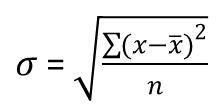
Where σ denotes the standard deviation
x represents the individual scores within the dataset
= the mean of the dataset (you will also meet contexts where it is appropriate to denote the mean with the Greek letter µ.
n = the number of scores in the dataset (You will also find that the capital letter N is used)
Remember that the Greek letter sigma (∑) means to“add together all the elements of a particular sequence/set.
The following table shows the heights is cm of two groups of people, group A and group B
| Group A | 160 | 160 | 160 | 175 | 180 | 170 | 160 | 165 | 155 |
|---|---|---|---|---|---|---|---|---|---|
| Group B | 180 | 160 | 230 | 160 | 170 | 165 | 125 | 150 | 145 |
a) Which group do you think would have the greatest range in heights?
b) Which group do you think would have the greatest standard deviation in heights?
c) Calculate these statistics for each group to confirm your prediction.
(You may either calculate the standard deviation by hand or using the statistics mode of your calculator or CAS calculator)
Click here to check your answer
Note:
Some important distinctions in relation to the standard deviation and the mean
The standard deviation calculations performed in the previous example, treated the standard deviation as a descriptive statistic.
Example
The standard deviation of 7.817 for group A is determined from how close each data value in the group A is to the mean value, we are not making any predictions about the larger population we are just finding the standard deviation of that particular group of data (as if it were the whole population).
It is often the case however, that we want to make predictions or inferences about statistics for a whole population from a sample from that population.
Suppose that our group A data is a sample from some wider population (although in reality the sample would be too small), and that we would like to use this sample to predict the mean and standard deviation of the population from which the sample was drawn. In this situation the formula for calculating the standard deviation is different and is given by:
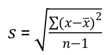
Note that the denominator is n-1 instead of n.
We use this formula when estimating the standard deviation of a population from a sample. The reason why the denominator is n-1 is complex but in essence it goes some way to correct for bias in the estimation of the population standard deviation from a sample.
It is also worthwhile pointing out some differences in notation, particularly as you may need to interpret equivalent representations of the formulae in the practise examples provided in a weblink further on.
In the first formula shown below, the mean and standard deviation are parameters (i.e., fixed numerical characteristics of a population), and the Greek letter µ is used to denote the population mean and the lower case Greek letter σ denotes the population standard deviation (that is, their true values). In the second formula shown below, the sample’s mean is denoted and the sample’s standard deviation is denoted by s (these are our estimates of the true values using the sample rather than the whole population).
1. The Population Standard Deviation: 
2. The Sample Standard Deviation: 
Notice also the equivalent notation where ![]() and
and ![]() taken to the left of the summation sign in formula 1 and 2 respectively are equivalent to:
taken to the left of the summation sign in formula 1 and 2 respectively are equivalent to:
The following link from Math Is Fun - Maths Resources provides an overview of the meaning of the standard deviation including the difference between the population and sample standard deviation. This is followed by some practise problems towards the end of the page.
The following section touches on the distinction between the population mean and the sample mean.
In many situations in statistics, the population mean µ, is an unknown parameter (in practical terms it may not be feasible to survey every single element or item within your population of interest). In this case, the sample mean , is an unbiased estimate of the population mean μ. This idea will be dealt with in more depth in particular aspects of your Health Science course work.
On the other hand, sometimes we might know the mean of the population we are interested in (e.g., from a previous census).
If we then draw a sample from the population, it might be helpful to compare the mean of our sample to the mean of the population.
In order to infer whether or not the means are significantly different from each other, you might carry out a statistical test called a ‘t-test’. These ideas including t-tests will also be covered in your future course work.
The normal distribution is symmetrical about the mean as shown in the histogram below showing the heights of a students.
Image: www.abs.gov.au/websitedbs/a3121120.nsf/home/statistical+language+-+measures+of+shape
When a histogram is constructed on values that are normally distributed, the shape of columns form a symmetrical bell shape. This is why this distribution is also known as a 'normal curve' or 'bell curve'.
The same distribution (Heights of students) has been represented below, as a 'normal curve' (or bell curve), where µ = mean, and σ = standard deviation.
Image: www.abs.gov.au/websitedbs/a3121120.nsf/home/statistical+language+-+measures+of+shape
It just so happens that many measurable quantities (e.g., height, weight, IQ, haemoglobin levels, measurement errors), have values that are "normally" distributed.
In the normal distribution there is a special relationship between the area under the distribution curve and the mean and standard deviation. About 68% of the area under the curve is contained within one standard deviation from the mean. That is, about 68% of all values will be within 1 SD of the mean value. The diagram below shows that in general:
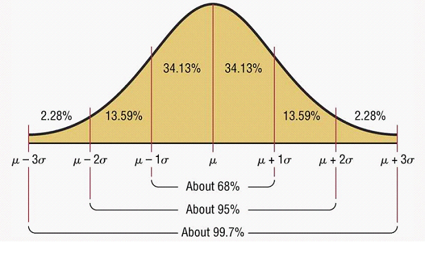
Image: rchsbowman.files.wordpress.com/2009/01/010309-1504-statisticsn2.png
Example
It is found that a population has an average resting pulse rate of 77 with a standard deviation of 12. We could therefore make the following statements:
About 68% of the population would have a pulse rate of between 65 and 89. Note that the mean pulse rate is 77 so 1 standard deviation either side of 77 is 65 and 89.
About 95% of the population would have a pulse rate of between 53 and 101.
About 99% of the population would have a pulse rate of between 41 and 113.
Almost all of the population would have a pulse rate of between 29 and 125.
A sample of women have height measurements with the mean of 170cm, σ = 5 cm, standard deviation 5cm tells us that:
Reaction times as measured in a psychology experiment, was found to be normally distributed with a mean of 0.40 seconds and a standard deviation of 0.03 seconds.
Complete the following statements:
1. We would expect that 68% of the people would have a reaction time of between___and___
2. We would expect that 95% of the people would have a reaction time of between___and___
3. We would expect that 99% of the people would have a reaction time of between___and___
4. We would expect that almost all of the people to have a reaction time of between___and___
Click here to check your answers
A confidence interval gives an estimated range of values which is likely to include an unknown population parameter, such as the population mean. If several independent samples are taken repeatedly from the same population, and a confidence interval is calculated for each sample, then a certain percentage of the intervals will include the unknown population parameter.
Confidence intervals are usually calculated so that this percentage is 95%, but we can produce 90%, 99%, 99.9% (or whatever) confidence intervals for the unknown.
A 95% confidence interval is often interpreted as indicating a range within which we can be 95% certain that the true effect lies. A more precise interpretation of a confidence interval is based on the hypothetical notion of considering the results that would be obtained if the study were repeated infinitely often, and on each occasion a 95% confidence interval calculated, then 95% of these intervals would contain the true effect (e.g., the true population mean).
The following video from the Statistics Learning Center explains some important concepts underpinning the concept of a confidence interval.
In a study of human blood types in nonhuman primates, a sample of 71 orang-utans were tested and 14 were found to be blood type B.
A researcher constructed a 95% confidence interval for the relative proportion of blood type B in the orang-utan population, (0.120, 0.305).
Interpret this interval.
Click here to check your answer
Positively skewed distributions have more than 50% of values below the mean (e.g., ages of 1st year nursing students at a particular university).
The tail of the distribution goes toward the positive end of the curve.
In a positively skewed distribution, the mean, median, and mode are not the same (as distinct from a perfect normal distribution where the mean, median and mode are equal).
In this case it is best to use the median or the mode as the measure of central tendency.
The figure below represents a positively skewed distribution curve:
The graph below shows a positively skewed distribution. In this situation, more people chose to retire when they were younger than the mean age.
Image: www.abs.gov.au/websitedbs/a3121120.nsf/4a256353001af3ed4b2562bb00121564/
445432b72bf470c7ca257b55002261e8/Body/3.3620!OpenElement&FieldElemFormat=gif
A bimodal distribution has two peaks in the distribution (2 different values that are very common) (e.g., the age distribution of patients in hospital - lots of young children and old people but not many 20 to 40 year olds).
The diagram below shows a bimodal distribution of salaries for a particular sample of lawyers.
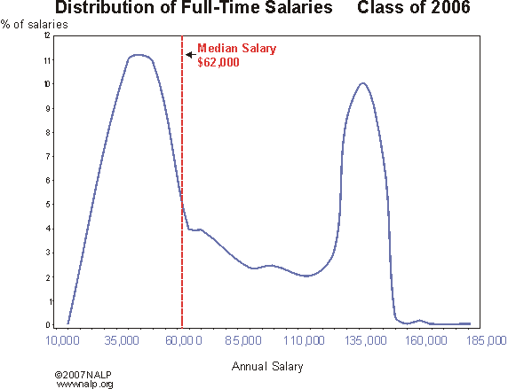
Image:1.bp.blogspot.com/-ojNwEP3f2b0/TtOop8h8y-I/AAAAAAAAAbU/Uv50Cjc1jZk/s1600/salaries.gif
The bimodal distribution below shows the frequency of body lengths of a sample of individual people. This sample tended to either have quite long bodies or fairly short bodies.
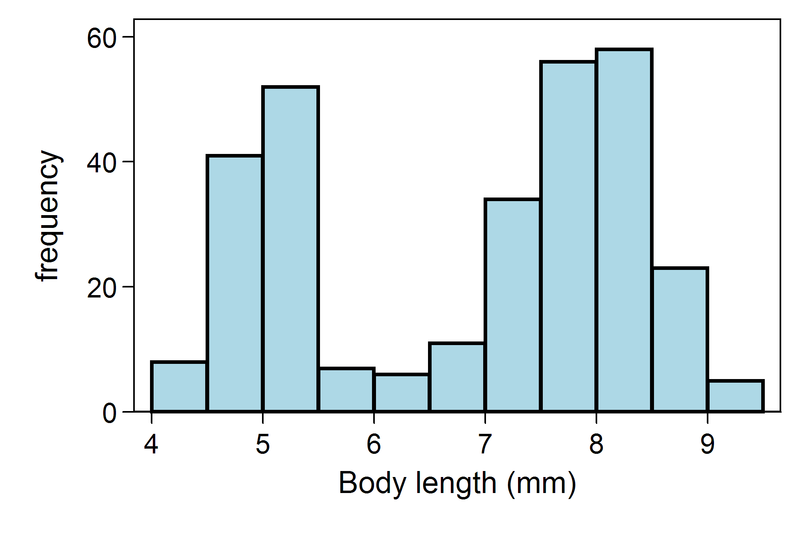
Image: upload.wikimedia.org/wikipedia/en/thumb/f/f2/BimodalAnts.png/800px-BimodalAnts.png
1. The median is a more appropriate measure of central tendency than the mean, when the distribution is:
A) SymmetricalB) SkewedC) NormalD) Bimodal
2. A normal distribution is best described when:
A) Researchers superimpose a smooth curve instead of a series of straight lines over a histogram.B) The tail of the distribution trails off to the left in the direction of the lower scores.C) The tail of the distribution trails off to the right in the direction of the higher scores.D) The large majority of scores are concentrated in the middle of the distribution and the scores decrease in frequency the further away from the centre they are.
3. A negatively skewed distribution is best described when:
A) The tail of the distribution trails off to the right in the direction of the higher values.B) The tail of the distribution trails off to the left in the direction of the lower values.C) The large majority of scores are concentrated in the middle of the distribution and the scores decrease in frequency the further away from the centre they are.D) The median is generally lower than the mean.
Click here to check your answers
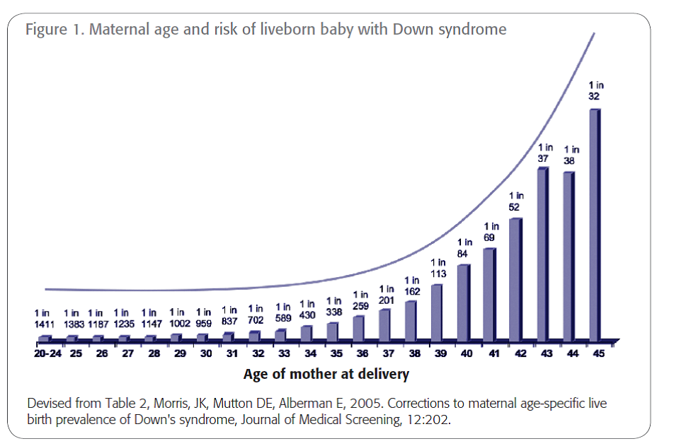 Image:w